Correlation risk arises when positions respond to the same market forces and lose together. Three trades on different assets may look diversified, yet amount to one larger bet. In binary options, that overlap matters because several losing contracts can each remove the full stake at expiry.
For Australian readers, this is an educational discussion, not a route to live trading. ASIC’s product intervention order bans the issue and distribution of binary options to retail clients until 1 October 2031. The examples below use hypothetical contracts and paper trading records to explain how shared exposure affects risk.
What Correlation Measures
Correlation describes how two sets of observations move together. For trading analysis, those observations are usually price returns over matching intervals, rather than the price levels themselves.
A positive correlation means returns tend to move in the same direction. A negative correlation means they tend to move in opposite directions. A reading near zero indicates little measured linear relationship during the sample.
The commonly used Pearson correlation coefficient runs from −1 to +1. The endpoints represent perfect negative and positive linear relationships; zero represents no linear relationship. These are the boundaries in the NIST definition of the correlation coefficient.
A coefficient of +0.8 does not mean that two assets move together on 80% of occasions. Nor does it mean that a trade has an 80% chance of winning. It summarises a relationship within historical observations, not the probability of a future contract outcome.
Direction also matters. If two assets tend to rise together, higher positions on both can share exposure. A higher position on one and a lower position on the other changes that exposure, but does not automatically create a reliable hedge.
Different Assets Can Still Represent the Same Bet
Counting symbols is a poor substitute for examining what could make positions lose. Holdings across the same industry, region or security type can remain concentrated despite having different names. This overlap is one of the problems covered in FINRA’s guidance on concentration in correlated assets.
Currency pairs provide a straightforward illustration. Consider three hypothetical positions opened for an overlapping period:
| Position | Required direction | Shared exposure |
|---|---|---|
| EUR/USD higher | Euro rises against the US dollar | Vulnerable to US dollar strength |
| GBP/USD higher | Pound rises against the US dollar | Vulnerable to US dollar strength |
| USD/JPY lower | US dollar falls against the yen | Vulnerable to US dollar strength |
All three positions express a view against the US dollar. A broad dollar rise could hurt the entire group, even though the trade directions include both “higher” and “lower”. Reading only the button labels would miss the common exposure.
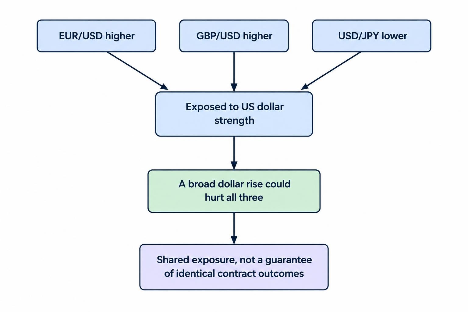
That does not mean these contracts must produce identical results. Movements in the euro, pound and yen also matter. The point is narrower: three symbols do not establish three independent risks.
Country Labels Do Not Remove Global Exposure
The same reasoning applies across asset classes and countries. A position linked to an Australian market is not insulated from overseas financial conditions simply because its label says Australia.
Global monetary policy and changes in investors’ appetite for risk can transmit into Australian financial markets. Australia’s floating exchange rate provides some insulation, not complete separation, as documented in the RBA’s research on global financial conditions and Australia.
For a paper portfolio, label the underlying assumption behind each position. “Australian shares higher” and “US shares higher” may both depend on the same improvement in sentiment. Different flags, same bet.
Price Correlation Is Not Binary Outcome Correlation
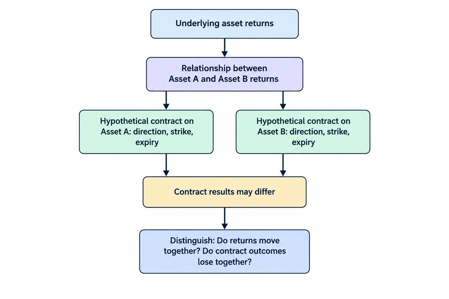
Binary options introduce a distinction that ordinary price charts can obscure. A relationship between asset returns is not the same as a relationship between contract results.
Two assets could rise together, yet a higher contract on one could win while a higher contract on the other loses. Their strikes may differ, their entry times may differ, or one asset may recover above its strike before settlement while the other falls short.
Consider two hypothetical higher contracts. Asset A starts at 100 and settles at 101. Asset B starts at 200 and settles at 201. Both assets rise. But if the contracts have strikes of 100 and 202 respectively, only the first wins.
Expiry matters too. A five minute contract and a thirty minute contract can settle on opposite sides of their strikes despite sharing part of the same market movement.
Assess correlation at two levels: the relationship between the underlying returns, and the tendency of the actual contract rules to produce joint losses. The second is closer to the account risk being managed.
A Worked Example: Three Stakes, One Exposure
Assume a hypothetical account contains A$1,000. Three overlapping contracts each carry a A$20 stake and offer an 80% net profit on a win. A winning contract returns the stake plus A$16; a losing contract loses A$20. Ignore fees, ties and early exits.
Each position risks 2% of the account. Together, however, they put A$60 at risk, or 6%. If all three lose, the account falls to A$940. If all three win, the combined profit is A$48.
The arithmetic does not care whether the positions appear on three separate charts. If the contracts depend on the same dollar move, their exposure belongs in one group before another stake is added.
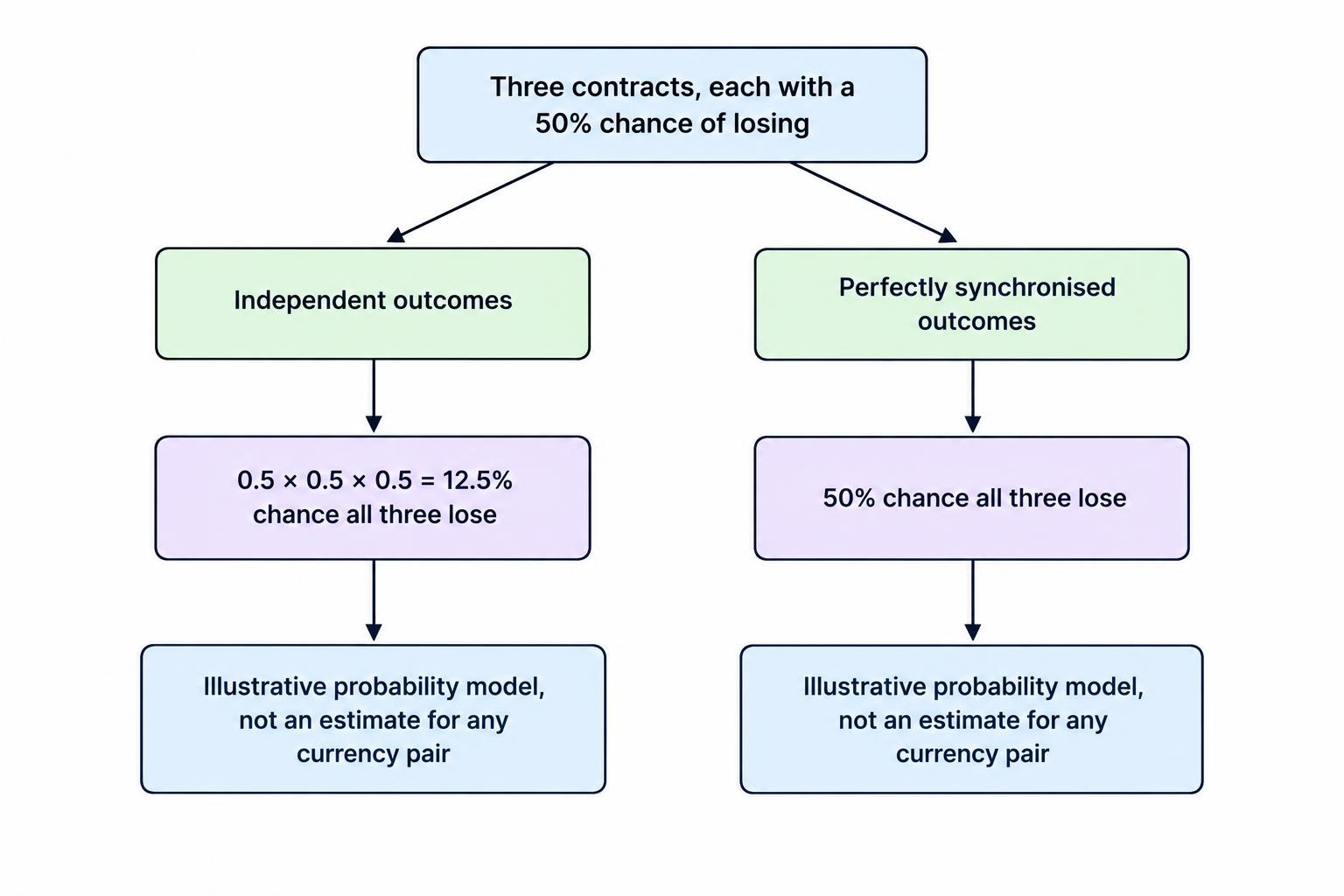
Now compare two simplified probability models. Suppose each contract has a 50% chance of losing:
- Independent outcomes: the probability that all three lose is 0.5 × 0.5 × 0.5, or 12.5%.
- Perfectly synchronised outcomes: if all three always win or lose together, the probability that all three lose is 50%.
These are illustrative endpoints, not estimates for any currency pair. They show why multiplying individual loss probabilities is wrong unless independence is justified.
A per-trade ceiling alone would miss this problem. Stake sizing needs to account for simultaneous exposure, not just the amount entered on each ticket.
Why Correlations Change
Historical correlation is a measurement, not a permanent property stamped onto an asset. Relationships can change when different forces take control of prices.
A growth surprise and an inflation surprise need not produce the same cross-market response. Monetary policy expectations can also change which force dominates. Long historical samples can blend together periods with quite different relationships.
Correlation has changed over time and sometimes switched sign across major financial markets. The RBA’s historical study of equity prices and government bond yields documents this variation and examines the roles of growth, inflation and monetary policy.
It would be wrong to turn that observation into “all correlations rise during stress”. Some relationships strengthen, others weaken, and some reverse. For risk control, the practical question is whether an assumed offset would still work under an adverse scenario.
A low average correlation should not be treated as permission to add more exposure without examining how the positions could fail together.
How to Assess Correlation in a Paper Portfolio
Match the Data to the Contract Horizon
Compare returns over matching timestamps and intervals. Daily observations do not directly answer a question about contracts lasting five minutes. Even five minute observations can mislead if one series closes its bars at different times from the other.
Keep the calculation consistent: the same sampling interval, aligned timestamps and a stated observation window. Check for missing quotes and periods when one market is closed. Otherwise, the result may partly describe mismatched data rather than a market relationship.
Use more than one observation window to see whether the reading is stable. A shorter window responds faster but contains fewer observations. A longer window contains more data but may mix different market conditions. Neither deserves automatic priority.
Record Joint Losses, Not Just Coefficients
For contract analysis, record the entry time, strike, expiry, direction, settlement rule and hypothetical result. Group overlapping positions and note whether they lost together.
A trading journal can then distinguish ordinary individual losses from losses concentrated around one event or market assumption. Include the common driver assigned before settlement, rather than inventing a neat explanation afterwards.
Keep separate records for different sessions and event conditions. Fifty contracts opened around one announcement are fifty records, but they are not fifty independent tests of the same idea.
Set Limits for Shared Exposure
A useful paper trading rule places a ceiling on each exposure group as well as on each contract.
Suppose a simulation allows no more than A$30 at risk on one shared market view. Two A$15 positions already use that allowance. A third correlated signal does not create another A$15 of capacity.
This A$30 figure is an illustration, not a recommended account allocation. The useful principle is that the group limit exists before signals appear and applies regardless of how many assets produce them.
When classification is uncertain, test a conservative grouping. Ask what happens if every overlapping position in the group loses. Do not reduce the assumed loss simply because a historical coefficient looks reassuring.
Also retain a ceiling on total open stakes. Correlation analysis can help identify concentration, but it should not replace the basic calculation of how much the account could lose across outstanding contracts.
Group Positions by Event and Expiry
Asset groups alone can miss exposure around an announcement. Several contracts might have different symbols and slightly different expiries, yet all remain open through the same data release.
Check the timeline. Which event occurs while the contracts remain open? Which positions depend on the same interpretation of that event? How much could be lost before any of them settles?
Staggering expiry times by a minute does not necessarily separate those risks. Event grouping connects correlation analysis with volatility and event risk, without assuming that a small timing difference creates diversification.
Why an Opposite Trade May Not Be a Hedge
An opposite direction can reduce exposure in some arrangements, but the contract terms must support the offset. A negatively correlated asset is not a guaranteed substitute for the original position.
Binary payouts also make apparent hedges expensive. Consider two A$20 contracts on the same underlying, strike and expiry, one higher and one lower. Assume identical settlement rules, no tie, and an 80% net profit payout on each.
One wins A$16 while the other loses A$20. The combined result is a A$4 loss. The uncertainty has been replaced with a known cost under those assumptions, not a profitable risk-free arrangement.
Different strikes can make matters worse. A higher contract with a strike of 100 and a lower contract with a strike of 99 would both lose if the settlement price were 99.5. Opposite buttons do not guarantee opposite outcomes.
Before treating any position as an offset, map both contracts’ results across possible settlement prices and times. If the supposed protection has gaps, those gaps belong in the risk assessment.
What Correlation Control Cannot Fix
Reducing dependence between outcomes does not turn unfavourable payouts into favourable ones. With fixed stakes, payouts and individual win probabilities, changing dependence changes the distribution of combined results, not their expected sum.
For example, assume a A$20 contract pays A$16 net profit on a win and has a hypothetical 55% win probability. Its expected result is:
(0.55 × A$16) − (0.45 × A$20) = −A$0.20 per contract.
Three such contracts have a combined expected result of −A$0.60, whether their outcomes are independent or move together. Correlation changes how those losses and wins can cluster. It does not repair the probability and expected value calculation.
Nor does spreading positions across assets remove a shared platform failure or settlement problem. Those are different risks and require separate checks.
Within binary options risk management, correlation analysis answers a focused question: how much apparently separate exposure could fail together? Start with the common market assumption, add the overlapping stakes, then test the joint loss. The number of charts open is not the number of risks held.
This article was last updated on: October 22, 2026